Modelling Chaotic Phytoplankton Behaviours
Phytoplankton may be tiny, but they run a huge part of the planet. Collectively, they contribute roughly half of Earth’s primary production [1]—meaning that about every second “bite” of new organic matter produced on Earth is made by them. Because phytoplankton sit at the base of marine food webs, phytoplankton also help steer the global cycles of carbon, nitrogen, phosphorus, sulfur, and many other compounds that climate and ecosystems depend on.
In the ocean’s sunlit surface layer (the euphotic zone), phytoplankton use photosynthesis to take up carbon and build biomass. That biomass is then eaten by zooplankton, which in turn are eaten by larger organisms. But not all of this material stays near the surface. Some of it sinks—either because phytoplankton clump together and fall like “marine snow,” or because zooplankton package it into fast-sinking fecal pellets. The result is a net transfer of carbon and nutrients from the surface to deeper waters. This conveyor belt of life and sinking particles is known as the biological pump [2]. It matters because it helps regulate how much CO₂ the ocean can store away from the atmosphere.
Despite the importance of phytoplankton for global biogeochemical cycles and cli mate, their composition and dynamics is still poorly understood. There are only few observations, and many species have not been identified or do not survive in culture. For example, recent research related to the TARA Oceans project showed a far larger diversity of eukaryotic phytoplankton than previously catalogued [3].

Fig. 1 Observations of the relative contribution of different phytoplankton to total biomass at the Santa Monica Bay station between 2004 – 2005 (source: Leinweber, A.).
At a single location—like the Santa Monica Bay station in Fig. 1—the relative contribution of different phytoplankton groups can swing dramatically over time. These jagged ups and downs naturally invite a provocative question: are phytoplankton dynamics chaotic—or are they simply responding to shifting conditions? On the other hand, fluctuations like those in Fig. 1 are not observed on large spatial scales, where external forcings like diffusion override the internal phytoplankton dynamics.
A Simple 1-D Model
This project tackles that question with a conceptual 1-D model designed by Scheffer [5]: a three-species food web where autotrophic phytoplankton (A) grow, herbivorous zooplankton (Z) graze them, and carnivorous zooplankton (C) snack on the grazers. The model was designed specifically to explore whether strange attractors might lurk behind plankton dynamics. The fun part is the experimental setup: first you let biology run the show (no vertical mixing), then you switch on vertical diffusion—a simple stand-in for the ocean’s habit of blending neighbouring layers together—and watch whether the “internal drama” survives.
The model lives in a 1D water column from 0 to 100 m, with daily time steps. Phytoplankton growth is strongest at the surface and decreases linearly with depth—basically a simplified “less light, less growth” rule:
r(z) = rmax · (1 − z/100)
So at 0 m, growth is maximal; at 100 m, it drops to zero.
Biologically, the equations include:
- growth and self-limitation for phytoplankton (A),
- grazing of A by herbivorous zooplankton (Z),
- predation of Z by carnivorous zooplankton (C),
- and mortality terms.
Grazing and predation follow saturating (Holling-type) functions so feeding doesn’t increase forever with prey abundance.
Numerically, the system is integrated with SciPy’s solve_ivp. Then comes the twist:
vertical diffusion is added using a seasonally varying mixed layer depth (MLD),
which sets a depth- and time-dependent diffusion coefficient
kz. In the report, diffusion is strongest near the surface and varies with an
annual MLD cycle (illustrated in Fig. 2).
Without Mixing
The first set of results is the “biology-only” experiment: each depth behaves like its own little ecosystem, only linked through the depth-dependent growth rate. In the depth–time maps (Fig. 3), phytoplankton generally decrease with depth—no surprise, since growth declines downward. But the pattern is not just a smooth fade. The result describes distinct vertical regimes: a high-A layer in roughly the upper ~40 m, then lower-density zones deeper down, with phytoplankton reaching deeper than the grazer and predator populations. More interesting: the system doesn’t behave the same everywhere. When the authors plot trajectories in 3D phase space (A–Z–C), they find different “personalities” at different depths during years 4–10. Around 40 m, the dynamics show deterministic chaos and evolve toward a strange attractor. At 62 m, behaviour looks like a limit cycle (repeatable oscillations). And at 68 m, the system tends toward a steady state (damped spiral settling). In this model, chaos is not a global personality trait—it’s a depth-specific mood.
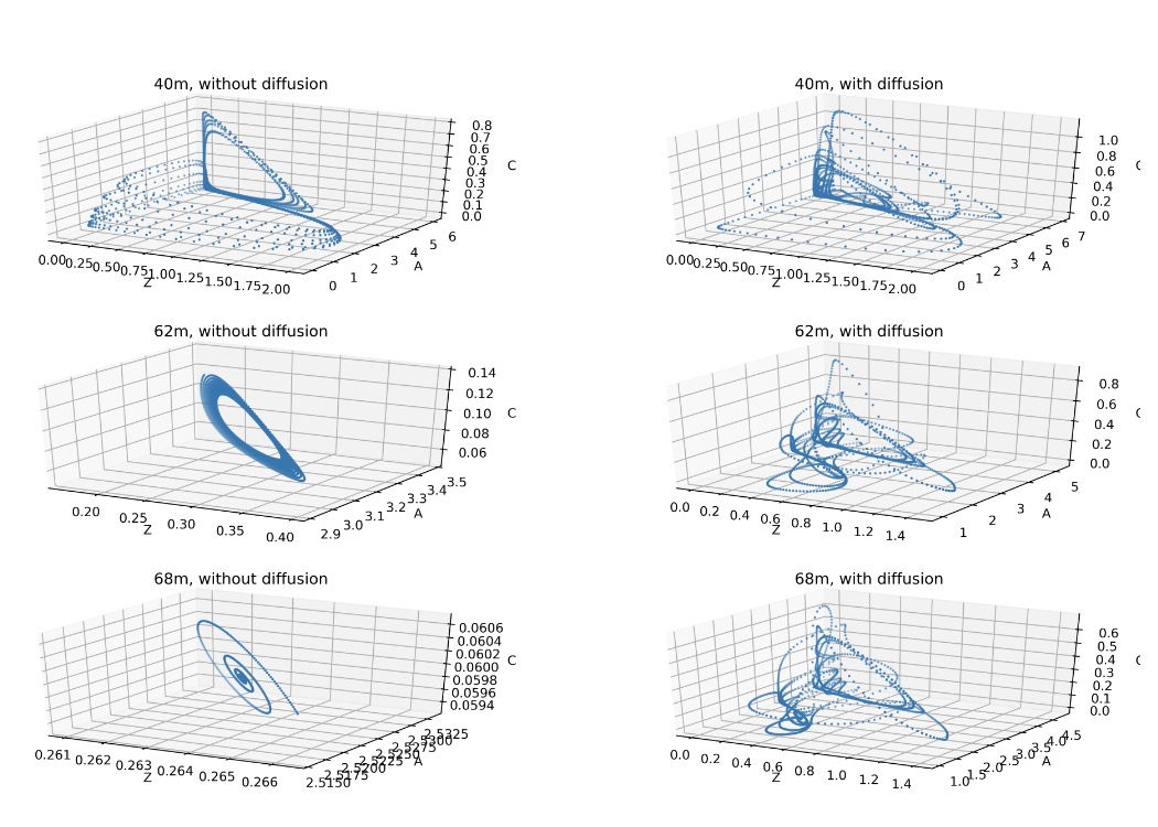
Fig.2 Plankton behaviour during years 4 to 10 in phase space without diffusion(left) and with diffusion(right).
Bifurcations
To make the “where does chaos come from?” question more systematic, we treat the phytoplankton growth rate r as a control knob and builds bifurcation diagrams. Without diffusion, there’s a clear transition around r ≈ 0.18 (about 64 m), where the system shifts from steady states to oscillations—consistent with a Hopf bifurcation.
Then another transition occurs around r ≈ 0.26, where the system moves into a strange-attractor regime (chaotic behaviour). You can literally see the system crossing a threshold where “boring and predictable” becomes “oscillatory,” and later becomes “chaotic-ish.” The takeaway is not “the ocean is chaotic everywhere,” but rather: simple predator–prey rules can generate complex behaviour once the system sits in the right parameter range.
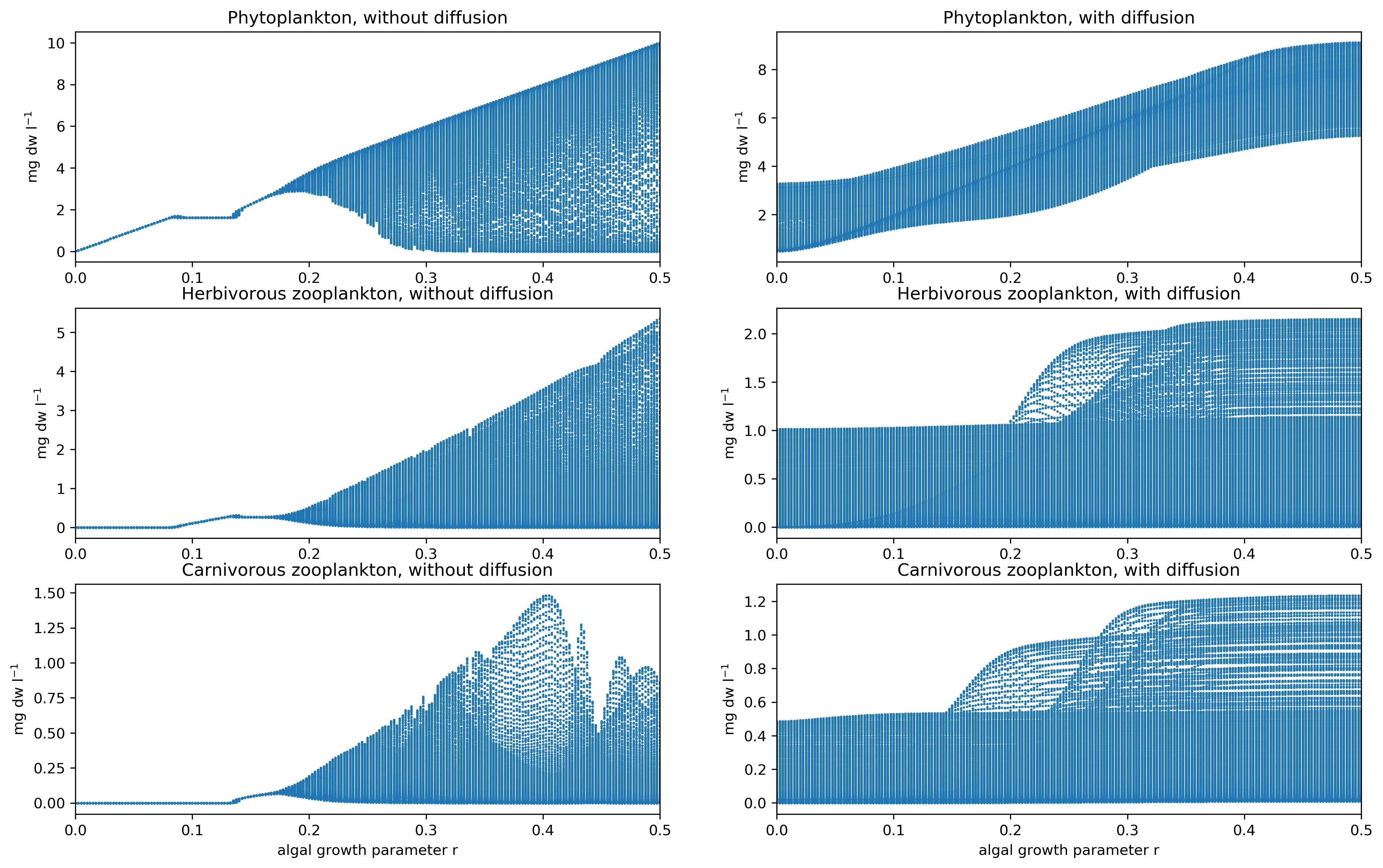
Fig.3 Plankton behaviour bifurcation diagram.
With Diffusion
Adding vertical diffusion changes the story dramatically. In the depth–time plots with diffusion, the cycles look more regular, and sharp boundaries between high and low concentrations become smoother. Diffusion links neighbouring depths, so no layer can “free-run” entirely on its own anymore.
The phase-space evidence is even more blunt: with diffusion, at the previously “special” depths (40 m, 62 m, 68 m), the report finds no clear strange attractor, no clean limit cycle, and no simple steady state—in other words, no strong indication of deterministic chaos in the same sense as the non-diffusive case. Diffusion is producing vertical smoothing that fundamentally alters (and effectively overrides) the internal dynamics.
A fun way to say it: biology can be a chaotic jazz solo—but diffusion is the sound engineer who turns down the feedback and keeps the whole concert from spiraling off-stage.
References
[1]Christopher B Field, Michael J Behrenfeld, James T Randerson, and Paul Falkowski. Primary production of the biosphere: integrating terrestrial and oceanic components. science, 281(5374):237–240, 1998.
[2] Jorge L Sarmiento and Nicolas Gruber. Ocean biogeochemical dynamics. Princeton University Press, 2006.
[3] Colomban De Vargas, St´ephane Audic, Nicolas Henry, Johan Decelle, Fr´ed´eric Mah´e, Ramiro Logares, Enrique Lara, C´edric Berney, Noan Le Bescot, Ian Probert, et al. Eukaryotic plankton diversity in the sunlit ocean. Science, 348(6237):1261605, 2015.
[4] JA Vano, JC Wildenberg, MB Anderson, JK Noel, and JC Sprott. Chaos in low dimensional lotka–volterra models of competition. Nonlinearity, 19(10):2391, 2006.
[5] M. Scheffer. Should we expect strange attractors behind plankton dynamics–and if so, should we bother? Journal of Plankton Research, 13:1291–1305, 1991.
[6] Horst Malchow Klaus Jurgens Lutz Becks, Frank M. Hilker and Hartmut Arndt. Ex perimental demonstration of chaos in a microbial food web. Nature Letters, 435:1226– 1229, 2005.